Benchmarking a decade of quantum computers with games
With Maria Aguado Yañez, Astryd Park, Haripriya Pettugani and Daniel Bultrini

How good are current quantum computers? There are many ways to benchmark them. Some focus on the small things, looking at the quality of individual qubits and gates. Some focus on the whole, running a process across a whole QPU to see how it operates as a single unit. Some try to do a bit of both.
Only one tries to be a game.
Quantum Awesomeness
In 2018, Google proposed a method to benchmark an entire quantum processor (QPU), and even determine whether it could do things beyond the reach of classical computers. This method is essentially based on running random circuits. They gave their proposal a name that they thought was very grand.
Inspired by this, I came up with another method based on random circuits in the same year, and I also gave it a very grand name: Quantum Awesomeness.
For me the intention was not just to be a benchmark, but to be one that anyone could easily understand. For this reason I also wanted the results to be playable as a game, so that people could gain an intuition about QPUs and how they compare just by playing the game.
Entangling qubits
A QPU is a collection of qubits, which are the quantum version of bits. Like bits, qubits take a value of 0 and 1 if you look at them. Unlike bits, they will do other more complex things when you are not looking at them.
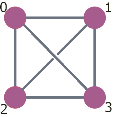
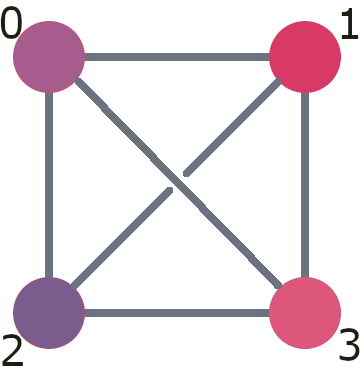
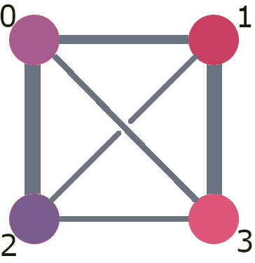
Qubits can be manipulated individually or in pairs in operations known as gates. Not all QPUs allow all possible pairs of qubits to interact, so the set of pairs for this allowed is an important feature of any QPU. For example, the following depicts four qubits (labelled from 0 to 3). The lines indicate which pairs allow a two-qubit gate. In this case we have all connected with all.
One of the basic features of quantum algorithms is the quantum phenomena known as entanglement. In the benchmarking we do here, we won’t consider any sophisticated use of entanglement. Instead we will look at how well the QPUs are able to manipulate it.
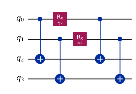
To create entanglement, it is usual to use a combination of single and two-qubit gates, such as those below.
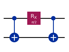
This is a diagrammatic depiction of a quantum program known as a quantum circuit. The gates that we apply are shown in order from left to right, with the black lines corresponding to different qubits. The two blue symbols denote a particular type of two-qubit gate, known as a CNOT gate. The box is a single qubit gate, applied to only one qubit, known as an RX. This is a gate that is controlled by a parameter. In the image above, this parameter has the value π/2. But in general we could use any value.
When we apply these gates to a pair of qubits, the end effect is that they become entangled. This means that, if we look at them, they will appear to be random and correlated. Specifically they will randomly take a value of either 0 or 1, but they will always agree.
By changing the parameter of the RX gate we can change how likely the qubits are to be 0 or 1. The qubits will be 0 with certainty if the parameter is 0, completely random for π/2 and 1 with certainty for π, with everything else somewhere in between.
Of course there are many more technicalities here. Such as what the CNOT and RX gates actually are, and how entanglement is more than just correlation of random bits. Nevertheless, we now have basically all we need to know to make a game.
Creating a puzzle
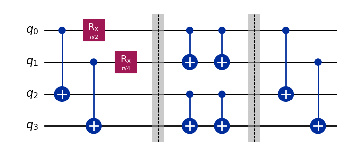
For our four qubits, let’s run the following circuit.
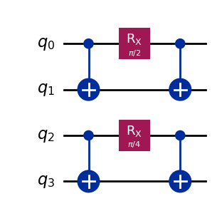
This entangles qubits 0 and 1 and also entangles qubits 2 and 3. For 0 and 1 the RX gate has π/2, so they both randomly take the value 0 or 1 with equal probability. For 2 and 3 the RX gate has π/4, so there is randomness but they are biased towards 0.
So suppose we ran this circuit many times, and used the results to measure the probability of getting a 1 on each qubit. For qubits 0 and 1 we will find that there is a 50% probability of a 1. For qubits 2 and 3 it will be more like 15%.
We can depict this with colour as in the image below. Here a qubit is shown as red if it will definitely come out 0, blue for definitely 1, purple for completely random and everything else is somewhere in between. So qubits 0 and 1 are purple, and 2 and 3 are mostly red.
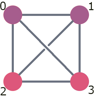
This is something that we could now present to people as a simple puzzle: Look at this image and find the pairs of circles. Two circles can only be paired up if they are connected by a line. The two qubits in each pair should be the same colour.
Creating another puzzle
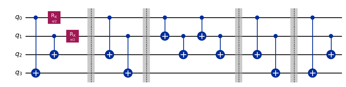
Now let’s create a puzzle with a different solution.
With this circuit it will be qubits 0 and 2 that are entangled with a parameter of π/2 and 1 and 3 entangled with π/2. So 0 and 2 would be purple, and 1 and 3 would be almost red.
However, suppose we ran this circuit instead.
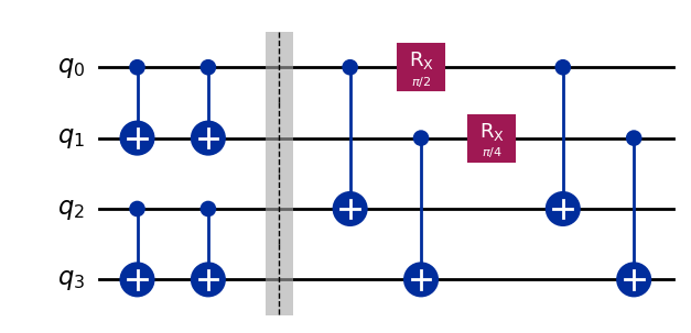
Here the dotted line doesn’t do anything, it is just there to separate two different parts of the circuit. The final part, shown on the right, is the part that entangles our qubits to create our new puzzle.
The part on the left is the same as we used for the first puzzle, with one important difference: the RX gates are missing. Without these gates, no entanglement is created in this part of the circuit. In fact, without the RX between the two CNOTS they will cancel each other out. This part of the circuit therefore won’t do anything at all.
In this case, you may wonder why I bothered to include them. The reason is that this is not just a game, but it is also about benchmarking. Any gate on a QPU will be at least a little bit imperfect, and those imperfections will build up as a circuit increases in size. Though these gates will do nothing on a perfect QPU, on a real one they will result in the qubits not doing exactly what they should, and hence the probabilities not being the values that they should be.
Now the colours don’t match exactly, making it a little harder to identify the correct pairs. In this way we can both give the QPU a harder test, and also increase the difficulty of the game.
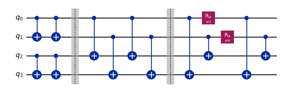
For Round 3 of the game we then continue this procedure. First we have the CNOTs from Round 1, then the CNOTs from Round 2, before finally actually creating the entangled pairs of Round 3.
So that we don’t make the game too hard for no reason, and give the QPU a chance to show what it can do, we should make sure to fully represent the data that we get. Rather than just look at the probability that each qubit gets a 1, we can also look at the probability that each pair of qubits agrees with each other. The entangled qubits should agree 100% of the time because they are fully correlated, whereas other pairs will only do it through random chance.
We can represent this in our game using the lines that connect pairs. Specifically, we’ll make the lines thicker when they have a higher chance of agreeing. For example, here’s the Round 2 puzzle from above with this new data.
Now Go Play!
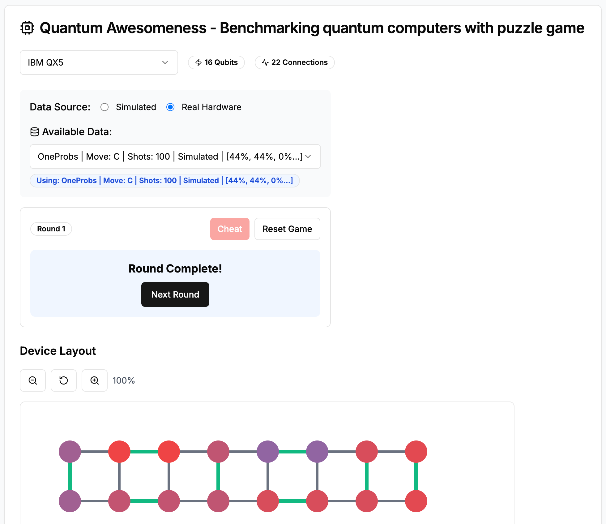
I have been running this process on QPUs for years now. I started in 2018 with IBM Quantum’s IBM QX2 and IBM QX4, both 5 qubit devices that were among the first to be available on the cloud. Then I looked at their 16 qubit devices from the following years, as well as 8 and 19 qubit hardware from Rigetti. After a few years off, I then looked at IBM Quantum’s new hardware with over 100 qubits.
All of this is online and available to play with. Unfortunately, the only way to play the game has always been with a Jupyter notebook. Not the funnest or most accessible experience!
Fortunately, this era is now over. Thanks to my colleague Astryd Park at MOTH, we now have an interactive web app to play with this data.
At the time of writing you can play a version with just the coloured circles (called oneProbs mode) and you can play a version with the line thickness (sameProbs mode).
Below we see an example of oneProbs mode on IBM Quantum’s first 16 qubit device. Click on the links to guess which ones are paired. It’ll turn green if you are right, and red if you are wrong. This example shows results when I simulated the process without any errors. Select the Real Hardware data to see what results from a real QPU looked like.
An even awesomer version
After playing the game, you will probably have opinions on whether it is a very good game. If you are a quantum researcher, you might also have opinions on whether it is a good benchmark. Though having lots of useless gates does allow errors to build up, and therefore show us how much of an effect they have, the circuits we use don’t really allow these errors to do their worst. With the CNOTs of previous round constantly undoing each other, the QPU never really strays far from its nice, comfortable initial state.
So how can we change that? There is one simple change that makes a great start. We can make sandwiches!
Specifically, rather than putting the useless gates at the beginning, we can put them in the middle.
The CNOTs of Round 1 still do nothing, and so this still just creates the entangled pairs for Round 2. But because they are in the middle, they now have the effect of making some entanglement that we wouldn’t otherwise get, before undoing it again.
For Round 3 we continue the sandwich, putting the CNOTs of Round 3 around those for Rounds 1 and 2.
By the middle of the circuit, this now generates some pretty complex entanglement that covers the whole device, before undoing it again and returning to just the pairs we want. These circuits therefore move further into the kind of complex many-qubit states that we actually need to do a quantum algorithm, and so are a much better test of the QPU in use. As such, I wish that I’d had this idea in 2018, and that Quantum Awesomeness had always been like this.
Nevertheless, there is no time like the present to make it better. So let’s make it even better, by also combining it with one of the standard metrics for quantum benchmarking.
Randomized Benchmarking
For the small scale, the most popular method is called randomized benchmarking (or RB). This runs a random sequence of gates, followed by a single gate that undoes the effect of the whole sequence. Since this final gate should return the qubits to their initial state, we can measure how often errors mess things up by seeing how often the qubits don’t return to this state. Or, stated more positively, we can see how often everything is perfect because the qubits do return to this state. Either way, by comparing sequences of different lengths and doing some maths, we can then measure the average error per gate.
Though RB works very well when benchmarking just one or two qubits, things can get complicated when trying to apply it to a lot more. Suppose you have 100 qubits, for example, and can apply any single or two-qubit gate you want. RB requires you to apply random 100-qubit gates, but an arbitrary 100-qubit gate is a pretty complicated thing. No QPU will give you that as part of its basic instruction set, meaning that you’ll need to painstakingly construct them from just the basic single and two qubit gates. Since many would be needed, and each carries a probability of an error, your 100-qubit gates would be almost guaranteed to fail in at least some small way on current and near-term quantum hardware. This would give a very bad impression of your QPU.
Motivated by this, people have looked into multiple ways to apply the principles of RB to a whole QPU. From our perspective the most interesting is probably also the simplest: Mirror RB.
Mirror Randomized Benchmarking
Rather than doing a random 100 qubit gate, how about we randomly do single and two qubit gates across 100 qubits. We could then build up sequences of these to do benchmarking in exactly the same way as normal RB. So why wouldn’t this work? There are three main reasons.
Random single and two qubit gates across 100 qubits is not the same thing as a random 100-qubit gate, and so certain assumptions made when mathematically proving the effectiveness of RB are not satisfied.
You still need to do the final gate which will invert all that came before it. This will be about as complicated as everything before, becoming as complex as an arbitrary 100-qubit gate for long sequences. A final gate that gets worse and worse as sequences get longer also doesn’t work well with the mathematical proofs.
RB uses the probability the circuit has been executed perfectly. For 100+ qubits on current and near-term hardware, something having gone wrong somewhere at some point in the circuit is almost an inevitability. You would therefore need far too many samples to find the probability of the rare moments of perfection.
Mirror RB fixes these issues by making sandwiches.
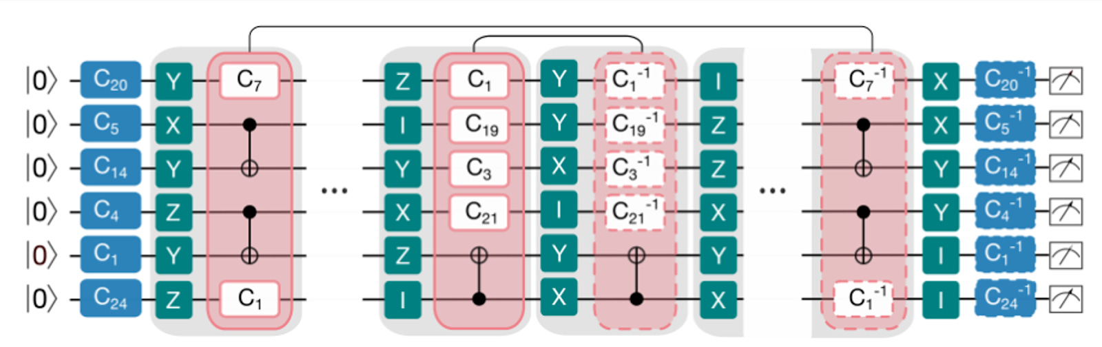
The image above is from the paper that introduced Mirror RB. On the far left we see some randomly chosen gates. They have been given nondescript names like C1 and C5. On the far right we see the inverses of these same gates, which are the gates that will exactly undo the effects of their counterparts.
The rest of the circuit is then composed of a sequence of blocks shown in grey boxes. These are random single and two qubit gates, with each box on the left mirrored by its inverse on the right. This is the principle with which Mirror RB circuits are constructed.
Another different to standard RB is that we no longer look at the probability that everything goes perfectly. Instead the authors define a new measure. This change, as well as the new structure of the circuit, doesn’t sit well with the original proofs for RB. However, the authors combine a mixture of new proofs and results from simulations to show that it works good enough.
Mirror Quantum Awesomeness
Given what we’ve learned about both Quantum Awesomeness and Mirror RB, the next step starts to become obvious: we need to do Mirror Quantum Awesomeness.
Essentially we just hijack the Mirror RB circuits, and insert some RX gates in the same place as we would for the sandwiched Quantum Awesomeness proposed earlier.
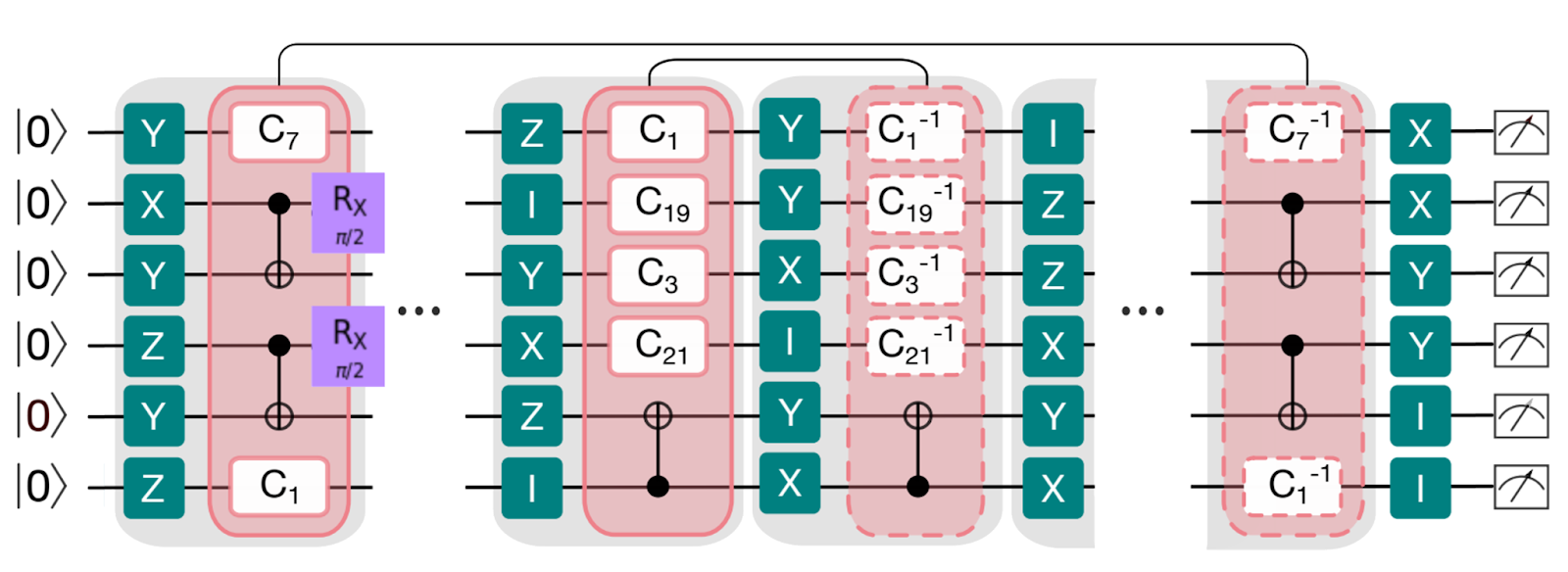
You might notice that we’ve also gotten rid of the gates to the far right and far left. This shouldn’t be too much of a problem. They are mostly there for Mirror RB because there is no reason why not to have them. For Mirror Quantum Awesomeness we do have a reason not to have them: they would make our entangled pairs give data that isn’t suitable for the game. So we get rid of them.
You might also notice some extra gates that we didn’t have in the sandwiched Quantum Awesomeness. The C gates don’t interfere with the entangled pairs we are creating, but they do mean that the entanglement generated by the middle of the circuit is even more complex than before. So our benchmark becomes even more representative of a QPU in action. They also scramble the noise to make it easier to measure.
The green gates are known as Paulis, and are essentially bit flips. They mean that the results at the end will not be quite the same as if they weren’t present, but this is easily fixed in post-processing. These circuits therefore allow us to perfectly merge the properties of Mirror RB and Quantum Awesomeness.
This is what MOTH Predoctoral Researchers Maria Aguado Yañez and Haripriya Pettugani, with help from MOTH researcher Daniel Bultrini, have been doing for the past few months: implementing this new form of Quantum Awesomeness, and testing both it and Mirror RB on the largest IBM Quantum devices. The details of all this will be explained in our upcoming paper. But for now, the most recent results have been uploaded to our new website. So have fun playing with Quantum Awesomeness!